There are several reasons why the evaluation of results on datasets like the Pascal-VOC and ILSRVC is hard. It is well described in Pascal VOC 2009 challenge paper.
Here are some of these:
Images may contain instances of multiple classes so it is not sufficient to simply ask, “Which one of the m classes does this image belong to?” and then use the predicted result to compare with the actual. There are multiple images and every image contains multiple classes- and the added dismay of accuracy for every image being a non-binary value.
Ok. How about a simple Accuracy measure (which checks the percentage of correctly classified exmaples)? Not Appropriate. Especially when in the sliding window method, it encounters thousands of negative (or background) examples for ever positive example.Because Accuracy = (TP + TN)/(TP + TN + FP + FN) and the number of TN’s would vastly overshadow the number of TP’s. Nay. Very Unbalanced.
The evaluation measure needs to be algorithm-independent; evaluation measures such as the Detection Error Tradeoff (DET) commonly used for evaluating pedestrian detectors is only applicable to sliding window methods and thereby constrained to a specific window extraction scheme, and to data with cropped positive test examples.
For this detection tasks, a number of bounding boxes are created by the rcnn with a confidence score attached to every bounding box. The NMS score is calculated for every bounding box to remove duplicates. If there are multiple bounding boxes detecting the same image, the bounding box with the highest confidence score is greedily selected.
A quick overview of Precision and Recall:
Suppose we are calculating Precision and Recall for the footballs detected. Precision is the percentage of true positives in the resultant bounding boxes. That is:
A note on Classification vs Detection
In the case of classification, whether an image is correctly classified or not depends on whether an image contains an instance of the target class or not. However, for detection purposes, the prediction must be based on where an instance of the class is present in the image. To this end, every detected bounding box was assigned to ground truth objects and judged to be a true or false positive based on the amount of overlap. To be considered a correct detection, the area of overlap a between the detected bounding box Bp and the ground truth bounding box Bgt must exceed 50% given by the formula:
Varying the confidence levels produces different values of precision and recall. If you increase the confidence threshold, the number of bounding boxes detected would be lesser but more precise.
As you relax the “threshold,” you will generally increase the proportion of true positives (more probable bounding boxes will be included) at the expense of including many more false positives (more distractors will be included). At the same time, the number of false negatives will decrease rather drastically.The precision will therefore decrease while the recall increases. There is therefore a trade-off involved between precision and recall, or equivalently, between the number of false positives and false negatives.
So what’s the next step? Drawing a Precision Recall Curve (by relaxing the confidence thresholds).
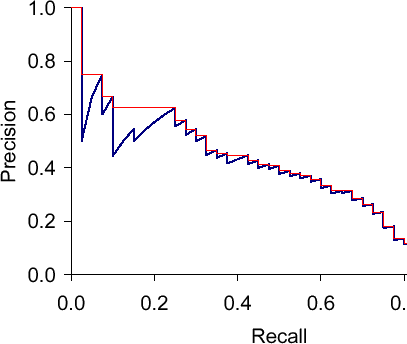
The area under this Precision-Recall curve gives you the “Average Precision”.
As you can see, the precision-recall curve contains a lot of “wiggles”. To reduce the amount of wiggles and smoothen the curve out to calculate an alternative approximation that is called “Interpolated Average Precision”. Instead of using the precision that was actually observed at cutoff k, the interpolated average precision uses the maximum precision observed across all cutoffs with higher recall. The full equation for computing the interpolated average precision is:
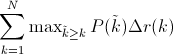
An easy way to visualize this is- start from the rightmost data point and take small steps (delta r) back. You look at all the precision values ahead of you in the right hand-side direction and choose the maximum encountered. The red line in the graph is indicative of the same.
To have a high score of AP or IAP- you need to have high precision at ALL levels of recall.
You can do a deeper level of analysis, by digging into the False Positives and False Negatives.
Let’s take a closer look at the False Positives.
In what cases can a False Positive occur?
Due to Localization error- when an object did not have a bounding box with the ground truth box overlap > 0.5 and was therefore considered as a false positive.
Confusion with similar objects- for example, a sofa detector may assign a high score to a chair. They are both said to be “similar” objects since they semantically belong to the same class- furniture.
Confusion with dissimilar objects- when the neurons are wildly misfiring! let’s say it mistook your face for a baboon.
Confusion with background -These could be detections within highly textured areas or confusions with unlabeled objects that are not within the class labels.
You can draw a simple pie chart to figure out which of these 4 cases is causing the majority of False Positives. Accordingly, the treatment must be decided.
Can you think of other things? Other possible errors and diagnoses?
Well, an interesting one- Looking at the size (big or small?) of the object may give you an idea on whether the object will be detected or not. Smaller objects have fewer visual features, it is more likely that they may not be detected. On the other hand, let’s say someone took a large close-up picture of your face and fed it to a person-detector. Sometimes such large objects have unusual viewpoints or are truncated making them hard to detect.